How to Price the Carbon Exposure of Any Business Jet Before You Finance It

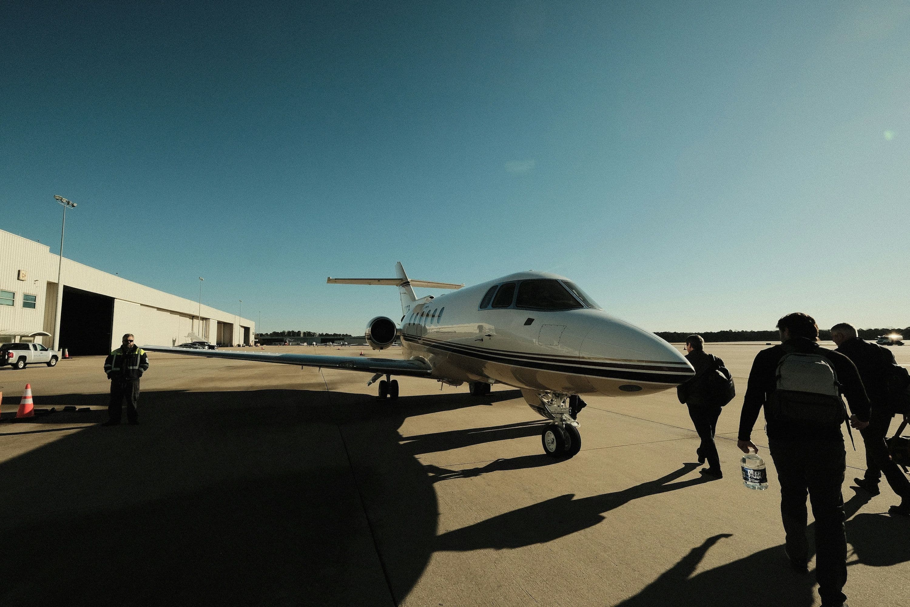
To show what the method surfaces, we modelled an 18-jet, large-cabin refinancing portfolio using observed fleet activity rather than manufacturer fuel-burn assumptions.
The result: a carbon assumption about 16% higher than the financing model carried — and a previously unpriced regulatory exposure of roughly €1.5 million a year.
The figures below are illustrative and internally consistent; the method behind them is exactly what you'd run on a real transaction. Here it is, in full.
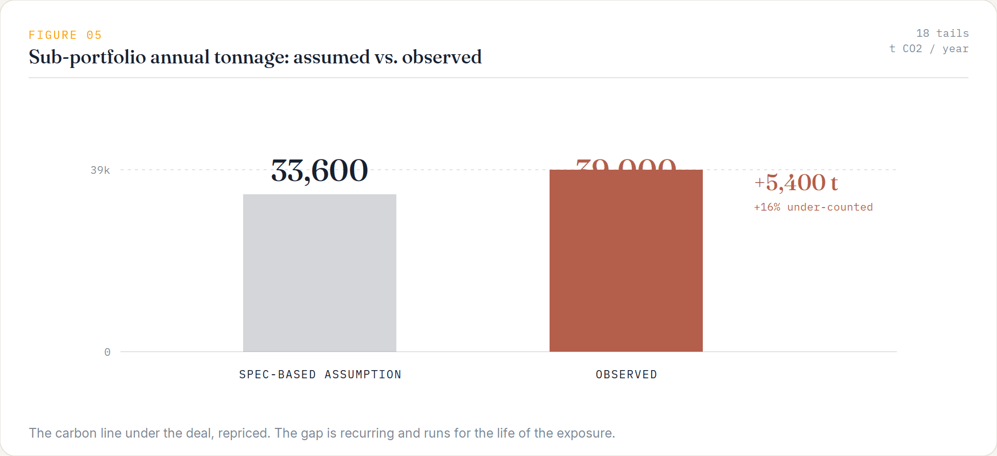
Figure 05 - assumed vs. observed annual tonnage, 18-tail sub-portfolio. Lead with this image: it's the result.
Carbon has become a finance input
For many business aviation operations, emissions now create direct compliance costs - through the EU ETS, the UK ETS, and, from 2027, CORSIA Phase 2 where applicable.
That turns carbon into a finance input: a recurring cost line under the asset for the life of your exposure, not a sustainability footnote. And the number most models use for that line is wrong - in a direction that costs you.
The deal, walked through
Anonymised and illustrative. Figures are internally consistent - to be replaced with the type's live Model Intelligence output.
The lessor was sizing the refinance on the manufacturer's cruise burn, applied flat across expected hours.
Two questions before committing: does that assumption hold against real behaviour, and what's the exposure under EU/UK ETS and CORSIA Phase 2?
The fleet. The total tracked fleet for the type stood at 472 tails, flying ~70,800 flights over the trailing year, well past coverage thresholds, so coverage completeness was high.
Mean utilisation was ~150 flights per tail, but the lessor's 18 sat in the upper half of the fleet's utilisation distribution — relatively high-utilisation aircraft. That distinction matters, because financing portfolios are rarely random samples of the global fleet.
The gap.
Observed emissions came out at ~5.0 tonnes CO₂ per hour, against the ~4.3 assumed - about 16% higher once applied across the 18 tails' real hours: roughly 39,000 tonnes a year instead of 33,600.
The hidden line.
Mapping routes, ~34% of that tonnage fell in EU ETS or UK ETS scope, and a further ~41% became CORSIA-eligible where applicable from 2027. At an assumed €80/tonne, the ETS-scope tonnage alone implied ~€1.1 million a year, with additional CORSIA exposure where applicable. Depending on route eligibility and applicable treatment, this produced the ~€1.5M line the financing model didn't carry.
What they did.
They folded the observed per-hour figure and the exposure band into their residual model at each tail's expected hours, repriced the carbon line, and put the 18 tails on a watchlist.
It didn't change whether they did the deal. It changed the number they did it at. That’s where the difference starts affecting pricing.
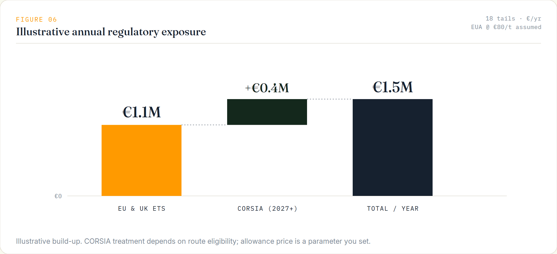
Figure 06 - regulatory cost exposure waterfall: ETS + CORSIA where applicable.
Why the manufacturer figure fails
So why is the manufacturer figure different?
Manufacturer fuel burn describes a clean-sheet mission flown at optimal weight and altitude. The real fleet doesn't fly that mission.
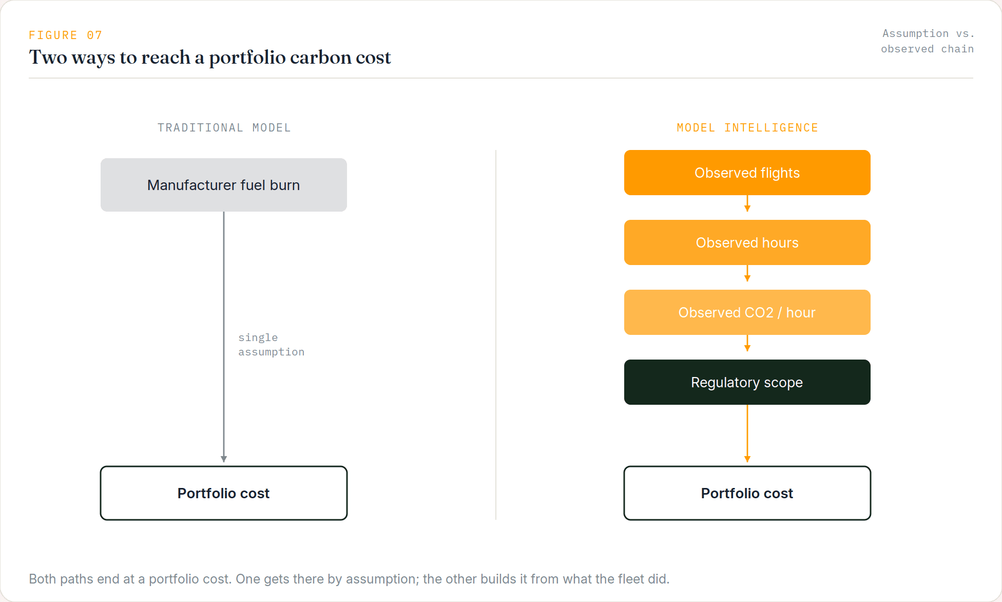
Figure 07 - traditional model vs. Model Intelligence: assumption leap vs. observed chain.
Three things pull it off:
Mission mix. Short missions typically produce higher emissions per flight hour, because the fuel-heavy climb is a larger share of total flight time. A jet certified for transatlantic range often lives on one- and two-hour legs.
Utilisation spread. Two fleets with the same average utilisation can carry very different portfolio risk, because the financed tails are rarely the average ones.
Route structure. Where a type flies decides which regime its emissions fall under — an empirical question, not an assumption.
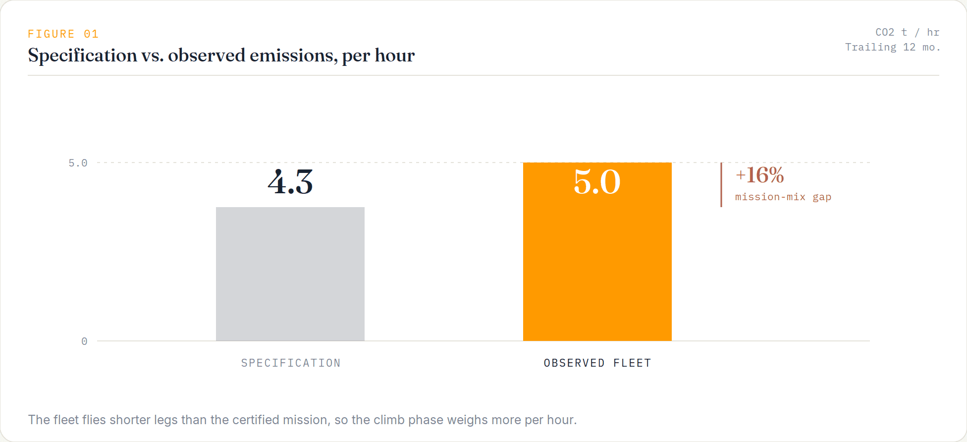
Figure 01 - specification vs. observed emissions per hour.
The method
None of these steps are unusual.
The methodology is public; producing reliable inputs at fleet scale is the difficult part.
In principle, any organisation could reproduce this workflow.
In practice, assembling global ADS-B coverage, matching aircraft consistently over time, maintaining the emissions calculations, and producing repeatable outputs at fleet scale is the engineering problem.
Model Intelligence provides that infrastructure, it removes the operational burden, not the underlying methodology.
The activity comes from ADS-B: each observed flight provides an origin, destination, date and duration, building a trailing-12-month activity record for each tracked tail.
Calculations use the published EUROCONTROL EMEP/EEA 2023 methodology, with fixed conversions and no smoothing or estimation.
How much you can lean on a figure depends on how completely the fleet is observed.
Coverage completeness is reported alongside the numbers: where ADS-B coverage of a type is thin, that's surfaced rather than smoothed over, so you know how much of the fleet's activity the figures rest on.
A Model Intelligence document assembles this automatically for any type with five or more tracked tails and 100+ flights a year.
Aircraft finance is priced at portfolio level. Carbon should be too.
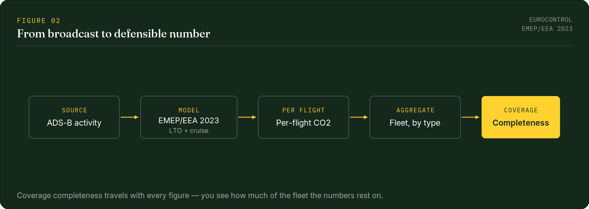
Figure 02 - method flow: ADS-B → EMEP/EEA 2023 → per-flight CO₂ → fleet → coverage.
What this can't tell you
Being explicit about the limits is what makes the rest defensible — so this comes before the how-to, not buried after it.
It won't tell you who owns or operates a tail, and it won't infer it. It produces no passenger counts and no invented fields.
Where coverage of a type is thin, that's surfaced as reduced completeness rather than papered over.
And it's an emissions and exposure input - not a valuation, and no substitute for your underwriting.
Those constraints are what make the output usable in front of a credit committee, an auditor, or a regulator.
That is the only setting where any of this is worth producing.
The seven steps
Step 1: Pull the whole tracked fleet
Take the full tracked population of the model, globally, not a sample. This is what separates a type assessment from an anecdote.
Output: tracked-tail count · trailing-12-month flights · coverage completeness.
The header states all three up front. A low completeness reading tells you how much of the fleet's activity the numbers below actually rest on.
Step 2: Establish the activity baseline
Get total flights, total hours, and how hours are spread across tails and not just the mean.
Output: total fleet hours · mean hours per tail · utilisation spread (median vs. top decile).
The utilisation panel shows where your financed tails sit. Upper-half tails carry more exposure than a fleet-mean assumption implies.
Step 3: Convert activity to emissions
Apply the model to get CO₂ per hour, per flight, and per year. Anchor on per-hour - it scales directly to a financed tail's expected hours.
Output: observed CO₂ per hour · per average flight · fleet annual tonnage.
The per-hour panel shows immediately whether observed behaviour diverges from the manufacturer assumption. It's the single most important number on the page.
If you take one number into your financial model, take observed CO₂ per flight hour.
Step 4: Map the regulatory scope
Classify flights by regime - EU ETS, UK ETS, CORSIA-eligible from 2027 - from origin and destination, not assumption.
Output: share of flights and tonnage under each regime.
The route-scope breakdown shows how much of the fleet's carbon already carries a price, and how much is about to.
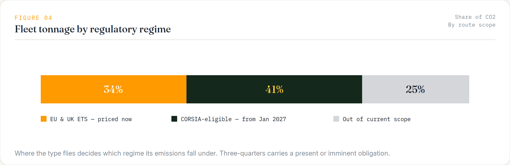
Figure 04 - fleet tonnage by regulatory regime.
Step 5: Quantify the exposure
Turn in-scope tonnage into a cost band. Set the allowance price as a parameter and show a range, not false precision. For this sub-portfolio's ETS-scope tonnage:
Allowance price
Annual ETS exposure
€65 / t ~€0.9m
€80 / t ~€1.1m
€95 / t ~€1.3m
Output: annual exposure band, per tail and at sub-portfolio level.
The exposure panel takes your allowance-price input and returns the banded cost - the line most financing models don't carry.
Step 6: Hand it to your model
The emissions profile and exposure band are inputs to your residual and underwriting work. They don't replace it. Drop the per-hour figure in at each tail's expected hours.
Output: per-tail emissions and exposure inputs, ready for your model.
The export gives you per-tail figures at the utilisation you specify, ready to drop straight in.
Step 7: Put it on a Watchlist
Your exposure runs for years; the snapshot shouldn't. Monitor the type and financed tails as the fleet keeps flying and parameters change.
Output: a live monitor for the life of the exposure.
With the type and your tails on a watchlist, the profile updates instead of freezing at close.
One application of many
Carbon exposure is one use of the same fleet record.
The trailing activity behind it also supports utilisation benchmarking and fleet-behaviour analysis across a type - the kind of inputs that sharpen your own aircraft residual value and underwriting work rather than replace it.
You've got the whole method. Run it on the type in front of you - open the Model Intelligence document, work Steps 2–5 against your sub-portfolio, set your allowance price, and put your tails on a watchlist to keep it live.